The topic is very new to me but being familiar to Databases is the reason I am exploring this concepts.. And in exploring the concepts I am going to use Mysql as my data support.
Before we begin with the technical things let us understand why we need to study Data Warehousing? What is the difference between typical RDBMS and Data Warehouse?
Little bit of googling can give you many answers. There is one basic difference between these two is that the data storage technique is little bit different in a DW as compared to RDBMS.
Generally, RDBMS are designed for transactional purposes whereas DW are designed for analysis purpose. And for analysis, the data from traditional RDBMS systems are Extracted, Transformed in a way which is best suited for analysis and then Loaded into the DW, also called ETL. Once you are done with ETL you are ready to go for analysis.
This is the basic difference known to me. You can add your answers in replies. So there are many things which we will be exploring one by one as and when needed. Let's have a glance at basic fundamentals(please go through the following terms from this link in case you find it difficult to understand) The contents of this post are borrowed from this link.
Star Schema is basically the database structure of DDW and Surrogate key is a column we need to add to DW table that acts as a primary key.
Fact table consists of facts(or measures) of the business and Dimension table contains the descriptions for querying the database.
There are many arrangements for Fact and Dimension table and one of them is "One Star Table" which has one Fact table and two or more than two Dimensional tables.
Here we are going to start with 4 little tasks.
1. Create a new user in Mysql environment.
2. Creating a relational database for DW and one Source database ( subject to ETL).
3. Creating tables for DW.
4. Generating Surrogate Keys ( please note unlike primary keys we do not enter values for surrogate keys, as we will make the system to generate one).
2. Creating a relational database for DW and one Source database ( subject to ETL).
3. Creating tables for DW.
4. Generating Surrogate Keys ( please note unlike primary keys we do not enter values for surrogate keys, as we will make the system to generate one).
Following are the snapshots for task 2 to 4. Creating a new user is hardly any challenge for SQL users.
Task 2

Task 3
.jpg)
.jpg)
.jpg)
Task 4
.jpg)
.jpg)
**End Of chapter 1**
********Chapter 2********
********Chapter 2********
In this chapter we are going to learn how to modify the dimension tables. Since DW is different from typical OLTP RDBMS w.r.t maintaining Dimension History, let us see how does it help us.
We will be dealing with two aspects of DW here. SCD1 and SCD2.
SCD1->Slowly Changing Dimension of type 1 in which the original data is replaced with the updated data and no track/history is maintained for the previous data.
SCD2->Slowly Changing Dimension of type 2 in which the original data is made history data by changing its expiry date to one day before the origination of new data and its entrance to the table. In this way the previous record is kept whereas the change is also reflected in form of new entry.
Applying SCD1 to customer_dim table where the customer name for customer_number=1 is changed from "Big Customers" to "Really Big Customers" and a new record is inserted. By definition of SCD1 we are not keeping any track of updation done.


Here we have two records in product_dim table. Snapshot is given below.

product_dim table. We will change the name of the product from Hard_Disk to Hard Disk Drive and we will insert one more record for LCD Monitors. Since we are changing the name we need to keep the track of previous record. Let us look at the following snapshot to understand how it is done.


**End of Chapter 2**
*******Chapter 3*******
Now we will discuss about additive measures. If you remember we have two types of tables i.e. fact table and dimension tables. So a measure is an attribute of fact table that is numeric and subject to arithmetic operations i.e sum, difference, avg, min, max etc. It can be fully additive as well as semi-additive.
Fully additive means you can sum the values of a measure in all situations and semi-additive means you can add up the values of the measure in some situations.
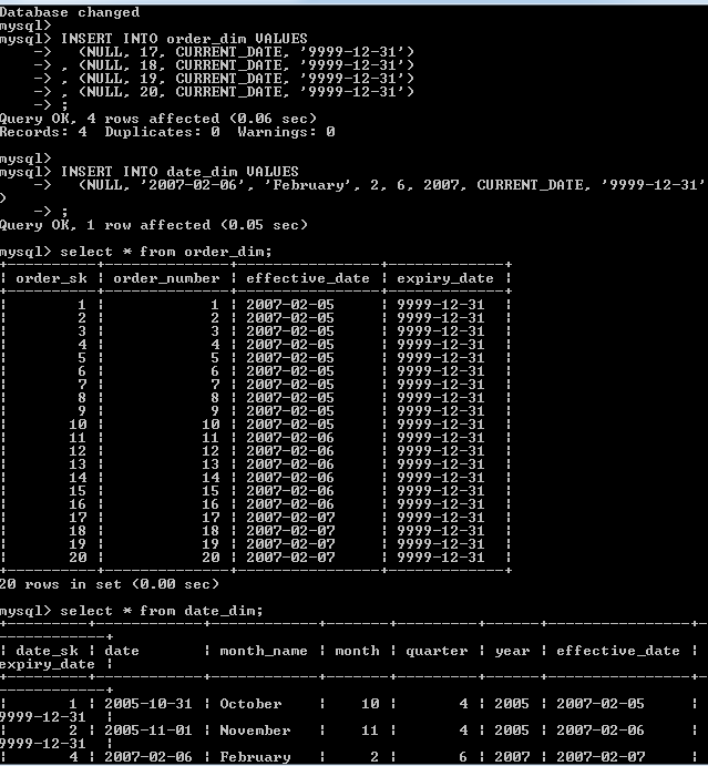
Before exploring the concepts of additive measures let us fill the tables
1. Order_dim
2. Date_dim
3. Sales_order_fact
Because there is no data in these tables. Following are the snapshots that explains how to fill in the data.


Now let us check for the whether the measure "order_amount" in sales_order_fact table is fully additive or not. It means it should give the same value every time a query is run on it. The query may be run on different table but it should show the same value every time. The total value of this measure should be Consistent.
1. Sum from the sales_order_fact. Sum is 58000

2. Sum from customer_dim. If we add all the values of sum_of_order_amount it will give 58000

3. Sum from product_dim. The values of the last column adds up to 58000

4. Sum from all the dimension tables. If all the values from the last column are added it turns up to 58000.

Clearly we can see the order_amount is fully additive.
**End of chapter 3**
*********Chapter 4**********
In this chapter we are going to query the dimensional data warehouse.
Before that let us insert few more records into
1
Order_dim
2
Date_dim
3
Sales_order_fact
The snapshot for the above data insertion is.


Now we will run the aggregate functions on these tables;
Here
we will run a query that give daily sales summary.

Now
we will look into the annual sales.

Specific Queries
A specific query selects and aggregates the facts on a specific
dimension value. The two
examples
show the application of dimensional queries in specific queries.
The query aggregates sales amounts and the
number of orders every month.

Quarterly
Sales in Mechanisburg
An another specific query. It
produces the quarterly aggregation of the order amounts in Mechanicsburg.

Inside-Out
Queries
While the preceding queries have dimensional constraints (the selection
of facts is based on
dimensions), an inside out dimensional query selects the facts based on
one or more
measure values. In other words, your query starts from the fact (the
centre of the star
schema) towards the dimensions, hence the name inside-out query. The
following two
examples are inside-out dimensional queries.
Product
Performer
The dimensional query gives
you the sales orders of products that have a monthly sales amount of 75,000 or
more.

Loyal Customer
The following query
is a more complex inside out query than
the previous one.. If your users would like to know which customer(s) placed
more than five orders annually in the past eighteen months, you can use the
query in. This query shows that even for such a complex query, you can still
use a dimensional query.

**End of chapter 4**
**********Chapter 5*********
This following chapter will deal with the ETL tasks. Extract, Load and Transform the data from source
tables(generally OLTP RDBMS tables) to Dimensional Data Warehouse tables.
Here we will do the Extraction and Loading parts. We need to
deal with which data we need to extract and load into DW tables.
Data can be extracted in two ways. “Whole Source” in which
all the records from the source tables are loaded into DW tables, and another one
is “Change Data Capture” in which only the new and changed records are loaded
since last extraction.
Direction of data extraction. “Pull by Data” in which the
source simply waits for the DW to extract it. “Push by Source” in which the
source pushes the data as soon as it is available.
Push-by-source CDC on Sales Orders Extraction
In this section we will look
on how push-by-source CDC works on sales order source data.
Push-by-source CDC means the
source system extracts only the changes since the last
extraction. In the case of
sales order source data, the source system is the source
database created in Chapter 1.
But before doing
any extraction we need to create tables in source database if you remember. So
lets create the sales_order table there.

Now let us write
a stored-procedure which we can run daily to extract the data from source
table.

Now let us
insert some records into order_dim and date_dim
Now we need to
insert some data into source table i.e sales_order table.

Now let us
switch to source database as we want to push the data from source to DW and we
will do that with the help of stored procedure written earlier.

**End of chapter 5**
*********Chapter 6**********
Populating
the date dimension
A date dimension has a
special role in dimensional data warehousing. First and foremost, a date
dimension contains times and times are of utmost importance because one of the primary
functions of a data warehouse is to store historical data. Therefore, the data
in a data warehouse always has a time aspect. Another unique aspect of a date
dimension is that you have the option to generate the dates to populate the
date dimension from within
the data warehouse.
There are three techniques to
populate data in date dimension.
The three techniques
are
·
Pre-population
·
One date everyday
·
Loading the date from
the source data
Pre-population
Among
the three techniques, pre-population is the easiest one for populating the date
dimension.
With pre-population, you insert all dates for a period of time. For example,
you
can
pre-populate the date dimension with dates in ten years, such as from January
1, 2005
to
December 31, 2015. Using this technique you may pre-populate the date dimension
once
only for the
life of your data warehouse.
the following snapshot shows a
stored procedure you can use for pre-population. The stored procedure accepts
two arguments, start_dt
(start date) and end_dt (end date). The WHILE loop in the stored procedure
incrementally generates all the dates from start_dt to end_dt and inserts these dates into the date_dim table.

One-Date-Every-Day
The second technique for
populating the date dimension is one-date-every-day, which is
similar to pre-population.
However, with one-date-every-day you pre-populate one date
every day, not all dates in a
period. The following snapshot loads the current date into the date_dim table.

Loading Dates from the Source
The following snap loads the
sales order dates from the sales_order
table in the
source database into the date_dim
table. We will use the DISTINCT keyword in
the script to
make sure no duplicates are
loaded.

Now let us add more records
to source sales order table and re run command.


**End of chapter 6**
**********Chapter 7**********
Initial Population
In chapter
6 we learned how to populate date dimension table. In this chapter we will
learn how to populate other dimension tables .
Clearing the tables

Pre-populating
the Date Dimension
call pre_populate_date ('2005-03-01',
'2010-12-31'); as we did in chapter 6. This procedure will populate the date dimension with all the dates between 01/03/2005 to 31/12/2010.
Preparing
the Sales Orders

Running initial population


**End of chapter 7**
**********Chapter 8**********
Regular Population
Regular population differs from initial population where the data is
loaded at one go whereas in regular population as name suggests populates the
data into tables from source tables on a regular basis.
Before running the Regular population codes, we need to load new data to
sales_order table of source.

Now let us run the scripts for loading data into dimension tables in "dw "database
using regular method.


Results to verify whether the data has been loaded into the respective tables or not.
Customer_dim table

product_dim table

**End of chapter 8**
chap 8.
ReplyDelete